Showing posts with label Maths. Show all posts

Tuesday 30 July 2024

New Video Posted: How to Calculate the Gradient (m) and Intercept (c) in y = mx + c | Gel Analysis Tutorial

This video is in response to a question I have received on YouTube:

“Thanks it is very helpful but can you present how to calculate slope and intercept in this curve”

The question often gets asked about two of my other videos:

In the How to Calculate the Gradient (m) and Intercept (c) in y = mx + c | Gel Analysis Tutorial, I explain how to calculate the gradient (m) and intercept (c) in the linear equation y = mx + c. I explain three methods that can be used:

  1. Graph-based calculation
  2. Solving simultaneous equations
  3. Using Excel or Apple Numbers.
In the video, I use DNA gel data to illustrate these calculations.

If you would like to say thanks for the video, then please feel free to buy me a coffee at https://www.buymeacoffee.com/drnickm

Blog Bonus: Free information sheet summarising the video and defining the key terms - download.

Additional Resources

Tuesday 14 May 2024

New eBook Available: Maths and Chemistry Refresher for Life and Biomedical Scientists

I have a new eBook available on Google Play Books - Maths and Chemistry Refresher for Life and Biomedical Scientists.

Maths and Chemistry Refresher for Life and Biomedical Scientists
Maths and Chemistry Refresher
for Life and Biomedical Scientists


The book is a refresher for life, biomedical sciences and chemistry students who may be a little unsure of some of the key maths and chemistry skill they need and covers:

  • Elements, atoms, ions, molecules, and compounds
  • Atomic weight, isotopes and molecular weight
  • Amounts, volumes, and concentrations
  • The SI units and the SI unit prefixes (m, ยต, n, p etc.)
  • Scientific Notation
  • Dealing with unit prefixes (m, ยต, n, p etc.) in calculations 
  • Order of operations (BODMAS and PEMDAS) in maths
  • How to get the best out of your calculator
  • Maths 'tricks' — Logs
  • And, graphs

Monday 6 May 2024

Mastering the Art of Graphing: A Step-by-Step Guide

Drawing graphs is essential in educational and professional settings, as it helps communicate information clearly and efficiently. Whether you're a student, a scientist, or just looking to present data compellingly, knowing how to create an effective graph is invaluable. Here’s a guide to help you draw graphs that are not only informative but also visually appealing.

1. Utilise Your Graph Paper Fully

The first step in drawing a graph is to make the best use of the available space on your graph paper. Avoid cramming all data into one corner; instead, spread out your data across the graph. This approach helps in better visualisation and interpretation later on.

2. Tools of the Trade

Always use a sharp pencil to mark points and draw lines. This ensures precision in your work, making your graph more readable and professional.

3. Plotting Your Points

Begin by placing your data points on the graph. Be precise and ensure each point is placed correctly according to the values it represents. This accuracy is crucial for the reliability of your graph.

4. Deciding on the Line of Best Fit

Once your points are plotted, decide whether to connect the dots directly or to use a line of best fit. If you opt for a line of best fit, ensure it appropriately represents the trend in your data, with the points evenly distributed around the line.

5. Drawing Lines

Whether connecting points directly or drawing a line of best fit, use a ruler to keep your lines straight and neat. For curves, maintain a smooth, consistent shape.

6. Labelling is Key

Clearly label your axes and include units of measurement. This step is crucial as it provides context to your data, making the graph informative and easy to understand. Remember to label both the x-axis and y-axis accurately. Don't forget the units.

7. Title Your Graph

Always give your graph a descriptive title that captures the essence of the data it represents. A well-chosen title can effectively communicate the purpose of the graph at a glance.

8. Setting Up Axes

Select sensible ranges for your axes to avoid data clustering that can occur if the ranges are too narrow. Proper scaling enhances the graph's clarity and makes it easier to interpret the data.

9. Interpreting Data

For instance, plotting a standard curve for protein concentration against absorbance, start with known concentrations on the x-axis and absorbance on the y-axis. Adjust the axis range to ensure all points are visible and not squished at the bottom.

10. Calculating and Using the Gradient

Once your graph is complete if you need to calculate the gradient of a straight line, draw the largest possible triangle under the line and use the formula (rise/run). This gradient could represent a specific value of interest, such as an extinction coefficient in spectrophotometry.

11. Dealing with Multiple Data Sets

If your graph contains multiple data sets, differentiate each set using various styles of points and lines. This distinction makes it easier to compare and contrast the data sets visually.

12. Avoid Extrapolation

Never extrapolate your data beyond the measured range. Doing so can lead to inaccurate conclusions. For data points that exceed the range of your graph, note that these values are beyond measured limits.

Final Thoughts

Graphing doesn't have to be daunting. With the right tools and a careful approach, anyone can create clear, informative, and visually appealing graphs. Remember, a good graph tells a story that speaks with clarity and impact.

If you would like to support my blogging efforts, then please feel free to buy me a coffee at https://www.buymeacoffee.com/drnickm

Blog Bonus: Free information sheet summarising the video and defining the key terms - download.

Additional Resources


Thursday 5 May 2016

What is the molarity of water?

An interesting little question and a fun bit of maths...

The molecular weight of water is: 18.02 g/mol

The density of water is 1 g/ml

Therefore, 1 litre of water (1000 ml) would weigh 1000 g

The molarity of something is the number of moles of that thing per 1000 ml volume.

So we have 1000 g of water in 1 litre, and the molecular weight is 18.02 g/mol

Now, let's calculate the molarity of water. We know that we have 1000 g of water in 1 litre, and the molecular weight of water is 18.02 g/mol. To find the number of moles, we divide the mass by the molecular weight: 1000 / 18.02 = 55.49 moles.

The 1000 g of water is in 1000 ml (1 litre), so the molarity of water is 55.49 M

You can also test your understanding of the above calculations at: Maths4Biosciences.

If you would like to support my blogging efforts, then please feel free to buy me a coffee at https://www.buymeacoffee.com/drnickm

Additional Resources

Thursday 10 April 2014

The importance of cell referencing in Excel spreadsheets...

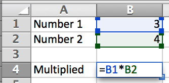
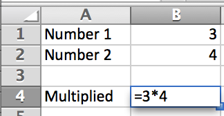
Using Excel correctly in the lab is an important skill to develop, and students sometimes get this wrong by failing to correctly use cell referencing and instead "hardcoding" key numbers into the formulas they are using. The consequence of doing this is that if the student later changes any of the numbers, these changes will not cascade through the spreadsheet, and this can lead to errors.

The video below demonstrates the importance of cell referencing and why it should be used as opposed to "hardcoding"...

The key points are:

  • When analysing scientific data, the only number that should be entered into the spreadsheet is the raw data
  • All calculations being performed should reference cells (e.g. A2) used for the calculations and not contain numbers (e.g. the number from cell A2

So this means that cells should be:

Correct

And not...

Incorrect


If you would like to support my blogging efforts, then please feel free to buy me a coffee at https://www.buymeacoffee.com/drnickm

Saturday 20 October 2012

Calculating Percentage Solutions

For some reason, percentage solution calculations cause students some problems. However, hopefully, once you have read this blog post, you should have a good understanding of percentage solutions and how to do the calculations.

If you want to practice your 'science maths', then have a look at Maths4Biosciences

What are percentage solutions?

A percentage solution is an amount or volume of something per 100 ml or 100 g of a solution. It is as simple as that. It is a percentage.

Why are they used?

Percentage solutions are a convenient and easy way to record solution concentrations. One advantage is that you don’t need to know anything about the compound in terms of molecular weight; all you need is the percentage of the required solution.

Why are there three types of percentage solutions?

This is slightly difficult to explain. However, there are three types of percentage solutions:
  • Percentage weight by volume (w/v)
  • Percentage volume by volume (v/v)
  • Percentage weight by weight (w/w)
The percentage weight by volume (w/v) is the number of grams of compound per 100 ml of solution. This type of percentage solution is used when describing the amount of powder in a solution. For example, 5 g of powder made up to a final volume of 100 ml would be a 5% (w/v) solution. Likewise, 2.5 g of powder made up to 50 ml would also be a 5% (w/v) solution, as you would have 5 g in 100 ml.

The percentage volume by volume (v/v) is the number of ml of some liquid per 100 ml of the solution. This type of percentage solution is usually used to describe a solution made by mixing two liquids. For example, 5 ml of a liquid made up to a final volume of 100 ml would be a 5% (v/v) solution. Likewise, 2.5 ml of a liquid made up to 50 ml would also be a 5% (v/v) solution, as you would have 5 ml in 100 ml.

Finally, the percentage weight by weight (w/w). This one is more difficult to understand, but the principles, as explained above, are still valid. A percentage weight by weight (w/w) solution can be the weight of a powder or a liquid made up in a solution to the final weight of the solution. So, for example, 5 g of a powder (or a liquid) made up in a solution with a final weight of 100 g would be a 5% (w/w) solution. Likewise, 2.5 g of a liquid or powder made up to give a solution that weighed 50 g would also be a 5% (w/w) solution, as you would have 5 g of the powder or liquid in 100 g of a solution.


If you would like to support my blogging efforts, then please feel free to buy me a coffee at https://www.buymeacoffee.com/drnickm

Additional Resources


Wednesday 6 October 2010

The Beer-Lambert Law, a straight line and the units of the extinction coefficient

If you would like to test your skills working with the Beer-Lambert Law, you might like to look at the Spectrophotometry tests at Maths4Biosciences.

Some students struggle to understand the relationship between the Beer-Lambert Law and a straight line and work out the units of the extinction coefficient (ฮต).

You may also find the following two videos helpful.


The Beer-Lambert Law states:

A = ฮต . c . l

Where:

A = absorbance 
ฮต = extinction coefficient 
c = concentration 
l = path length (i.e. the distance the light travels through the sample)


So, what is the connection between this and a straight line, and what are the units of the extinction coefficient?

The units of the extinction coefficient

In my opinion, the extinction coefficient has some of the craziest units out there.
Absorbance (A) has no units, so the units of the extinction coefficient (ฮต) are determined by how the concentration (c) and path length (l) are being measured. That is, the units of the extinction coefficient must cancel out the concentration and path length units so that the absorbance can have no units!

A worked example.

A = ฮต . c . l

A = absorbance, units - so put in 1 
ฮต = extinction coefficient, units - unknown 
c = concentration, units - milli-Molar, mM 
l = path length (i.e. the distance the light travels through the sample), units - cm

So...

A = ฮต . c . l

And, with units:


[1] = ฮต . [mM] . [cm]
Rearranging...
[1] / ฮต = [mM] . [cm] 

ฮต = 1 / ([mM] . [cm]) 

or 

ฮต = [mM]-1 . [cm]-1


So, the units are mM-1 . cm-1

This can be checked by putting it all back together:


A = ฮต . c . l 

A = ([mM]-1 . [cm]-1) . [mM] . [cm]

This gives:


A = [mM]/[mM] . [cm]/[cm]

So, the mM and the cm cancel each other out, leaving no units for absorbance A.

A straight line

The Beer-Lambert Law:

A = ฮต . c . l

Where:

A = absorbance 
ฮต = extinction coefficient 
c = concentration, units 
l = path length


The equation for a straight line is:

y = mx + c

Where:

m = the gradient 
c = the y-intercept

If you plot concentration against absorbance, then x = concentration and y = absorbance. Plus, from the Beer-Lambert Law, we know that if the concentration is zero, then absorbance must be zero.

A = ฮต . c . l
A = ฮต . 0 . l
A = 0 
So...

y = mx + c
absorbance = m . concentration + c

From above, if concentration = 0, then absorbance = 0, hence c must be zero
y = mx + c
absorbance = m . concentration + c*
0 = m . 0 + c 
c = 0

(* note, this c is the y-intercept and not the concentration)

Therefore...
y = mx + c
absorbance = m . concentration + 0
or
y = mx


Comparing:

y = mx
absorbance = m . concentration

With (and rearranging):

A = ฮต . c . l 

A = (ฮต . l) . c 

y = m . x
If y = absorbance, and x = concentration, then m (the gradient) must equal extinction coefficient (ฮต) multiplied by the path length, l, or ฮต . l. As l is typically 1 cm, the gradient, m, must equal the extinction coefficient (ฮต).

If you would like to support my blogging efforts, then please feel free to buy me a coffee at https://www.buymeacoffee.com/drnickm

Additional Resources

Thursday 11 March 2010

What is a Unit of enzyme?

What is a 'Unit' of enzyme.... this always seems to give problems.

1 Unit of enzyme is defined as "an amount of protein that produces 1 ยตmole of product per minute". The thing that causes the problem is the word "amount".

The "amount" is not a mass; it is, for want of a better word, a 'blob'. You can buy enzymes in 'Units'. You buy a vial that will contain a number of Units of enzyme. You then know that if you dissolve the contents of the vial in a solution, how many ยตmoles of product per minute will be produced. If you buy 1 Unit of a particular enzyme from two different suppliers you may have vials that contain different weights of powder, but the work that can be done (i.e. the amount of product produced) will be the same.

For example:

Look at these two 'piles' ('blobs') of enzyme:

One unit

Pile 1 of Enzyme

One unit1
Pile 2 of Enzyme

Both 'piles' contain the same number of red balls (i.e. 4), and if 4 red balls are needed to produce 1 ยตmole of product per minute (i.e. 1 Unit), then both piles can be said to contain 1 Unit of the enzyme, and yet, as you can see, there are many more balls in pile 2... Pile 1 is certainly more pure as there is less contaminant (yellow balls) around.

This is why the 'amount' in "an amount of protein that produces 1 ยตmole of product per minute" is not a weight; it is an 'amount'; it is a 'pile', a 'blob'.

If you have problems with 'Sciences Maths' then you might like to check out some of the courses over at Maths4Biosciences.

If you would like to support my blogging efforts, then please feel free to buy me a coffee at https://www.buymeacoffee.com/drnickm

Additional Resources


Friday 11 December 2009

Why did I get my standard deviation calculation wrong?

A number of the class members have asked why (or how) they calculated the standard deviation incorrectly in the assessment.

Having looked at the class answers it would appear that the main reason students got it wrong is because they were calculating the standard deviation of a POPULATION and not of a SAMPLE.

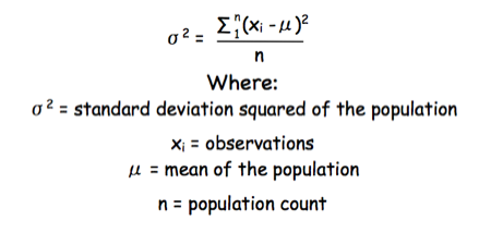
The equation for the standard deviation of a population (remember a population is ALL possible examples of a measurement/object and is something that is normally difficult to measure - think of the apple example in the lecture - as all examples can't be collected) is:

Standard deviation of a population

Equation for the standard deviation of a population

Whereas the standard deviation of a sample (which is what we had) is calculated by:

Standard deviation of a sample

The equation for the standard deviation of a sample

Note that the real differences between the two equations are that in the calculation of the standard deviation of a population, we are using the true population mean (ยต), whereas in the calculation of the standard deviation of a sample, we are using an estimate of the mean (x bar), plus in the calculation of the standard deviation of a sample we are using n - 1 (also called degrees of freedom) as this gives better estimate of the true standard deviation of a population (and we are working with a sample).

If you would like to support my blogging efforts, then please feel free to buy me a coffee at https://www.buymeacoffee.com/drnickm

Additional Resources

Tuesday 1 December 2009

How many molecules of X are there in a band on a Western Blot?

One of the questions I have often enjoyed setting in western blotting assessments, and that always seems to give problems, is...

"You have set up a western blot in which you wish to estimate the amount of GLUT4 per 3T3-L1 adipocyte (the cultured cell line used in the practical). You know that a 35 mm culture dish contains 2 million cells, and gives 1.5 mg total protein. You also have a recombinant stock of GLUT4 at 50 ng/ml. On your gel you load 15 ยตg of protein from the 3T3-L1 adipocytes and 1, 5, 10 and 20 ยตl of the GLUT4 stock. After probing with antibodies, you have a 55 kDa band in the 3T3-L1 adipocyte lane and in the GLUT4 stock lane. The band in the 3T3-L1 adipocyte sample has the same intensity of band as the 10 ยตl GLUT4 stock. How many molecules of GLUT4 are there per adipocyte?"

The chances are you are getting 'freaked out' by all the weird numbers flying around. The answer is to go back to basics.

For example:

If you had something with a molecular weight of 10, and you loaded 5 g on a lane, you would have 0.5 moles in that lane.

You know how many molecules there are in a mole (it is a constant that is the number of atoms in 12 g of carbon 12), so that constant multiplied by the number of moles would be the number of molecules in the lane.

Let's say one mole of something contains 100 molecules (which it doesn't; the real number is much, much bigger).

So, if you have 0.5 moles in the lane, you would have 50 molecules in that lane.

If you have another lane with a known number of cells in, say, 25, and that lane has the same intensity of staining as the lane containing 50 molecules, you could say that lane also has 50 molecules.
These 50 molecules came from 25 cells, so each cell must have 2 molecules.....

Now you can work it through with 'simple' numbers. All you need to do is to plug in the 'complicated' numbers in the question...

If you struggle with 'Science Maths' then you may like to look at Maths4Biosciences

If you would like to support my blogging efforts, then please feel free to buy me a coffee at https://www.buymeacoffee.com/drnickm

Additional Resources

Monday 2 November 2009

Deriving Lineweaver-Burk Reciprocal Plot from Michaelis Menten Equation II

OK, well, here is another way Deriving Lineweaver-Burk Reciprocal Plot from Michaelis Menten Equation, this time starting from a different point (the other approach is here)...


Enzymes equation


Where E = enzyme; S = substrate; ES = Enzyme substrate complex; and P = product

The Michaelis-Menton Equation given in your lectures describing the reaction is:


Eq2 2 1


Where v = rate (initial velocity); Vmax = maximum velocity (100% of enzyme catalytic sites occupied); Km = Michaelis constant (concentration of substrate to achieve half Vmax); S = substrate concentration

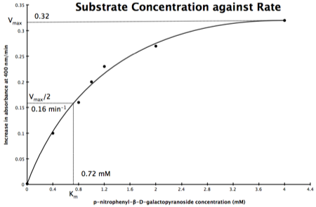
In the lab we can change the substrate concentration (S) in a reaction and measure the rate (v). As you know, a plot of substrate concentration (S) against rate (v; initial velocity) gives a curve, which plateaus at Vmax, with Km the concentration at half-Vmax:


Substrate concentration against rate


Plot of Substrate Concentration against Initial Velocity (rate)

The direct measurement for Vmax can never be achieved in the lab as the concentration of the substrate needed would never be reached. Also, in the lab we would use a computer to calculate the values, and determine Vmax, and Km. However, you should be able to calculate Vmax, and Km yourself, just so you know the computer is right, and it is possible calculate these values from experimental data by using a linear plot and an equation derived from the Michaelis-Menton Equation.

As you know, the equation for a straight line is:


Equation 1


Equation for a straight line, where m = the gradient and c = the intercept on the y-axis
So, the problem is, how do we get:


Eq2 1


to look like equation 1 so we can plot a straight line using the terms we can measure, i.e v and S? The answer is, we rearrange....

The first thing we need to do is invert equation 2 to get:


Eq2 3


If you didn’t understand that ‘mathematical move’ consider this:

Equation 4


The above is true. That is, 2 over 1 = 2, 4 over 1 = 4 and 2 times 4 is 8. If I simply invert (flip) all the parts:


Equation 5


It is also true.

Equation 3 is getting closer to what we want as we now have 1/v and this is our y in equation 1. All we need to do now is ‘extract’ x (which is our substrate concentration) from equation 3.

So, we have:


Eq2 4


which is the same as:


Eq2 5

If you consider the following it is true:


we can ‘separate terms’ on this and express it in several other ways:


Equation 12

That is, once we find a ‘common’ element (in the above example 1/2, and in equation 5 1 over [S]Vmax) we rearrange, so:


Eq2 5


extracting 1 over [S]Vmax in equation 4 we get:


Eq2 6


multiplying through with 1 over [S]Vmax gives:


Eq2 7


As you can see in equation 6 we have two terms after the + that can cancel out, and our experimental variable (S) can be separated, so:

/div>
Eq2 8


so we get:


Eq2 9


If that bit of maths has lost you, consider this:


Equation 9


if you divide both sides by 2 it is still correct:


Equation 10


However, on the righthand side the two 2s can be cancelled to give:


Equation 10a


which is still correct.

Finally, separating out 1/[S] from 7 gives:


Eq2 10


Which when compare to equation 1:


Equation 19


It can be seen that:
  • y = 1/v
  • x = 1/[S]
  • c, the y intercept = 1/Vmax
  • m, the gradient = Km/Vmax
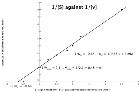
And, the intercept for the x axis, (i.e. when rate (y) = 0) is 1/-Km.

Hence, the final graph is:


Lbgraph


If you struggle with 'Science Maths' then you may like to look at Maths4Biosciences

If you would like to support my blogging efforts, then please feel free to buy me a coffee at https://www.buymeacoffee.com/drnickm


Additional Resources

Sunday 1 November 2009

Deriving Lineweaver-Burk Reciprocal Plot from Michaelis Menten Equation I

After a recent seminar, a number of students have asked how to derive the Lineweaver-Burk Reciprocal Plot equation from the Michaelis Menten equation... so, here goes.

The enzymatic reaction can be viewed as:

Enzymes equation

Where E = enzyme; S = substrate; ES = Enzyme substrate complex; and P = product

Blog Bonus: Free PDF of this blog post - download.

The Michaelis-Menton Equation describing the reaction is:


Michaelis menton


Where v = rate (initial velocity); Vmax = maximum velocity (100% of enzyme catalytic sites occupied); Km = Michaelis constant (concentration of substrate to achieve half Vmax); S = substrate concentration

Now, if the equation you are starting with does not look like the one above then have a look at another post (apparently I do it the 'old fashioned way’!)

In the lab, we can change the substrate concentration (S) in a reaction and measure the rate (v). As you know, a plot of substrate concentration (S) against rate (v; initial velocity) gives a curve, which plateaus at Vmax, with Km the concentration at half-Vmax:


Substrate concentration against rate

Plot of Substrate Concentration against Initial Velocity (rate)

The direct measurement for Vmax can never be achieved in the lab as the concentration of the substrate needed would never be reached. Also, in the lab, we would use a computer to calculate the values and determine Vmax, and Km. However, you should be able to calculate Vmax, and Km yourself, just so you know the computer is right, and it is possible to calculate these values from experimental data by using a linear plot and an equation derived from the Michaelis-Menton Equation.

As you know, the equation for a straight line is:


Equation 1

Equation for a straight line, where m = the gradient and c = the intercept on the y-axis

So, the problem is, how do we get:

Equation 2

to look like equation 1? The answer is, we rearrange....

Rearranging

We need to 'extract' our substrate concentration S and our rate v so we can plot them on a straight-line graph. Basically, we need to get equation 2 to look like equation 1.

The equation for a straight line is:

Equation 1

And our Michaelis-Menton Equation:

Equation 2

So, the first thing we need to do is invert equation 2 to get:

Equation 3

If you didn’t understand that ‘mathematical move’ consider this:

Equation 4

The above is true. That is, 2 over 1 = 2, 4 over 1 = 4 and 2 times 4 is 8. If I simply invert (flip) all the parts:

Equation 5

It is also true.

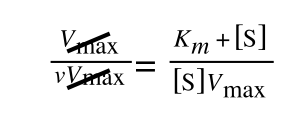
Equation 3 is getting closer to what we want. However, the Vmax over v is a problem as we don’t know Vmax and can only measure v and S in the lab. Therefore, we need to separate out the terms we can measure so we can have x and y as in equation 1.

To ‘remove’ the Vmax from the lefthand side we need to divide both sides by Vmax:

Equation 6

Note the new Vmax term on both sides of the equation - compare to equation 3.

As we now have Vmax over v multiplied by Vmax we can cancel out both Vmax:

Equation 7

to give:

Equation 8


If that bit of maths has lost you, consider this:

Equation 9

if you divide both sides by 2 it is still correct:

Equation 10

Blog Bonus: Free PDF of this blog post - download.

However, on the righthand side the two 2s can be cancelled to give:

Equation 10a

which is still correct.

In equation 5 we now have 1/v and this is our y in equation 1. All we need to do now is ‘extract’ x (which is our substrate concentration) from equation 5.

If you consider the following it is true:

Equation 11

we can ‘separate terms’ on this and express it in several other ways:

Equation 12

That is, once we find a ‘common’ element (in the above example 1/2, and in equation 5 1 over [S]Vmax) we rearrange, so:

Equation 13

extracting 1 over [S]Vmax we get:

Equation 14

multiplying through with 1 over [S]Vmax gives:

Equation 15

As you can see in equation 7 we have two terms after the + that can cancel out, and our experimental variable (S) can be separated, so:

Equation 16
Equation 17

Finally, separating out 1/[S] gives:

Equation 18

Which when compare to equation 1:

Equation 19

It can be seen that:
  • y = 1/v
  • x = 1/[S]
  • c, the y-intercept = 1/Vmax
  • m, the gradient = Km/Vmax
And, the intercept for the x axis, (i.e. when rate (y) = 0) is 1/-Km.

Hence, the final graph is:


Lbgraph


If you struggle with 'Science Maths' then you may like to look at Maths4Biosciences

If you would like to support my blogging efforts, then please feel free to buy me a coffee at https://www.buymeacoffee.com/drnickm

Blog Bonus: Free PDF of this blog post - download.
 

Additional Resources