The enzymatic reaction can be viewed as:


Now, if the equation you are starting with does not look like the one above then have a look at another post (apparently I do it the 'old fashioned way’!)
In the lab, we can change the substrate concentration (S) in a reaction and measure the rate (v). As you know, a plot of substrate concentration (S) against rate (v; initial velocity) gives a curve, which plateaus at Vmax, with Km the concentration at half-Vmax:
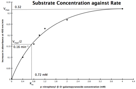
The direct measurement for Vmax can never be achieved in the lab as the concentration of the substrate needed would never be reached. Also, in the lab, we would use a computer to calculate the values and determine Vmax, and Km. However, you should be able to calculate Vmax, and Km yourself, just so you know the computer is right, and it is possible to calculate these values from experimental data by using a linear plot and an equation derived from the Michaelis-Menton Equation.
As you know, the equation for a straight line is:

So, the problem is, how do we get:

to look like equation 1? The answer is, we rearrange....
Rearranging
We need to 'extract' our substrate concentration S and our rate v so we can plot them on a straight-line graph. Basically, we need to get equation 2 to look like equation 1.
The equation for a straight line is:

And our Michaelis-Menton Equation:

So, the first thing we need to do is invert equation 2 to get:

If you didn’t understand that ‘mathematical move’ consider this:

The above is true. That is, 2 over 1 = 2, 4 over 1 = 4 and 2 times 4 is 8. If I simply invert (flip) all the parts:

It is also true.
Equation 3 is getting closer to what we want. However, the Vmax over v is a problem as we don’t know Vmax and can only measure v and S in the lab. Therefore, we need to separate out the terms we can measure so we can have x and y as in equation 1.
To ‘remove’ the Vmax from the lefthand side we need to divide both sides by Vmax:

Note the new Vmax term on both sides of the equation - compare to equation 3.

Where E = enzyme; S = substrate; ES = Enzyme substrate complex; and P = product
Blog Bonus: Free PDF of this blog post - download.
The Michaelis-Menton Equation describing the reaction is:

Where v = rate (initial velocity); Vmax = maximum velocity (100% of enzyme catalytic sites occupied); Km = Michaelis constant (concentration of substrate to achieve half Vmax); S = substrate concentration
Now, if the equation you are starting with does not look like the one above then have a look at another post (apparently I do it the 'old fashioned way’!)
In the lab, we can change the substrate concentration (S) in a reaction and measure the rate (v). As you know, a plot of substrate concentration (S) against rate (v; initial velocity) gives a curve, which plateaus at Vmax, with Km the concentration at half-Vmax:

Plot of Substrate Concentration against Initial Velocity (rate)
As you know, the equation for a straight line is:

Equation for a straight line, where m = the gradient and c = the intercept on the y-axis

to look like equation 1? The answer is, we rearrange....
Rearranging
We need to 'extract' our substrate concentration S and our rate v so we can plot them on a straight-line graph. Basically, we need to get equation 2 to look like equation 1.
The equation for a straight line is:

And our Michaelis-Menton Equation:

So, the first thing we need to do is invert equation 2 to get:

If you didn’t understand that ‘mathematical move’ consider this:

The above is true. That is, 2 over 1 = 2, 4 over 1 = 4 and 2 times 4 is 8. If I simply invert (flip) all the parts:

It is also true.
Equation 3 is getting closer to what we want. However, the Vmax over v is a problem as we don’t know Vmax and can only measure v and S in the lab. Therefore, we need to separate out the terms we can measure so we can have x and y as in equation 1.
To ‘remove’ the Vmax from the lefthand side we need to divide both sides by Vmax:

Note the new Vmax term on both sides of the equation - compare to equation 3.
As we now have Vmax over v multiplied by Vmax we can cancel out both Vmax:
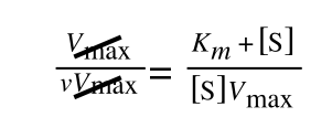
to give:


to give:

If that bit of maths has lost you, consider this:

if you divide both sides by 2 it is still correct:

However, on the righthand side the two 2s can be cancelled to give:

which is still correct.
In equation 5 we now have 1/v and this is our y in equation 1. All we need to do now is ‘extract’ x (which is our substrate concentration) from equation 5.
If you consider the following it is true:

we can ‘separate terms’ on this and express it in several other ways:

That is, once we find a ‘common’ element (in the above example 1/2, and in equation 5 1 over [S]Vmax) we rearrange, so:

extracting 1 over [S]Vmax we get:

multiplying through with 1 over [S]Vmax gives:

As you can see in equation 7 we have two terms after the + that can cancel out, and our experimental variable (S) can be separated, so:


Finally, separating out 1/[S] gives:

Which when compare to equation 1:

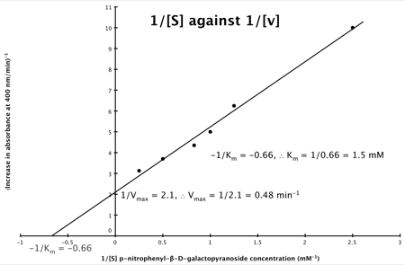
It can be seen that:
Hence, the final graph is:
if you divide both sides by 2 it is still correct:

Blog Bonus: Free PDF of this blog post - download.

which is still correct.
In equation 5 we now have 1/v and this is our y in equation 1. All we need to do now is ‘extract’ x (which is our substrate concentration) from equation 5.
If you consider the following it is true:

we can ‘separate terms’ on this and express it in several other ways:

That is, once we find a ‘common’ element (in the above example 1/2, and in equation 5 1 over [S]Vmax) we rearrange, so:

extracting 1 over [S]Vmax we get:

multiplying through with 1 over [S]Vmax gives:

As you can see in equation 7 we have two terms after the + that can cancel out, and our experimental variable (S) can be separated, so:


Finally, separating out 1/[S] gives:

Which when compare to equation 1:

It can be seen that:
- y = 1/v
- x = 1/[S]
- c, the y-intercept = 1/Vmax
- m, the gradient = Km/Vmax
Hence, the final graph is:

If you struggle with 'Science Maths' then you may like to look at Maths4Biosciences
If you would like to support my blogging efforts, then please feel free to buy me a coffee at https://www.buymeacoffee.com/drnickm
Blog Bonus: Free PDF of this blog post - download.
Additional Resources
- 📗 - Biochemistry (Stryer) (affiliate link to the book)
- 📗 - Principles of Biochemistry (Lehninger) (affiliate link to the book)
- 📗 - Maths and Chemistry Refresher for Life and Biomedical Scientists
- 📗 - Catchup Chemistry (affiliate link to the book)
- 📗 - Catchup Maths and Stats (affiliate link to the book)
Thanks for this derivation Nick, superbly explained and very easy to follow!
ReplyDeleteJust what I needed - Thanks
ReplyDeletegreat explanation
ReplyDeleteThank you, this is great
ReplyDeleteThank you, this is great
ReplyDeleteVery helpful thank you
ReplyDeleteWONDERFUL! it couldn't be more clear, great job!
ReplyDeleteThank you Nick👏
ReplyDeleteThnk u
ReplyDeleteThanks so much
ReplyDelete