Where E = enzyme; S = substrate; ES = Enzyme substrate complex; and P = product

Where v = rate (initial velocity); Vmax = maximum velocity (100% of enzyme catalytic sites occupied); Km = Michaelis constant (concentration of substrate to achieve half Vmax); S = substrate concentration
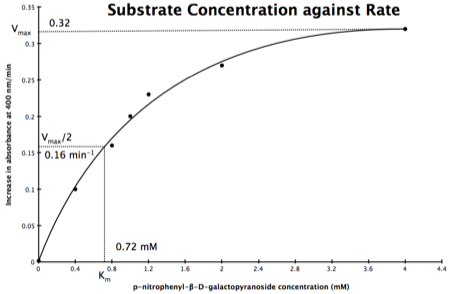
In the lab we can change the substrate concentration (S) in a reaction and measure the rate (v). As you know, a plot of substrate concentration (S) against rate (v; initial velocity) gives a curve, which plateaus at Vmax, with Km the concentration at half-Vmax:

Plot of Substrate Concentration against Initial Velocity (rate)
The direct measurement for Vmax can never be achieved in the lab as the concentration of the substrate needed would never be reached. Also, in the lab we would use a computer to calculate the values, and determine Vmax, and Km. However, you should be able to calculate Vmax, and Km yourself, just so you know the computer is right, and it is possible calculate these values from experimental data by using a linear plot and an equation derived from the Michaelis-Menton Equation.
As you know, the equation for a straight line is:

Equation for a straight line, where m = the gradient and c = the intercept on the y-axis
So, the problem is, how do we get:

to look like equation 1 so we can plot a straight line using the terms we can measure, i.e v and S? The answer is, we rearrange....
The first thing we need to do is invert equation 2 to get:

If you didn’t understand that ‘mathematical move’ consider this:

The above is true. That is, 2 over 1 = 2, 4 over 1 = 4 and 2 times 4 is 8. If I simply invert (flip) all the parts:

It is also true.
Equation 3 is getting closer to what we want as we now have 1/v and this is our y in equation 1. All we need to do now is ‘extract’ x (which is our substrate concentration) from equation 3.
So, we have:

which is the same as:

If you consider the following it is true:
we can ‘separate terms’ on this and express it in several other ways:

That is, once we find a ‘common’ element (in the above example 1/2, and in equation 5 1 over [S]Vmax) we rearrange, so:

extracting 1 over [S]Vmax in equation 4 we get:

multiplying through with 1 over [S]Vmax gives:

As you can see in equation 6 we have two terms after the + that can cancel out, and our experimental variable (S) can be separated, so:
/div>

so we get:

If that bit of maths has lost you, consider this:

if you divide both sides by 2 it is still correct:

However, on the righthand side the two 2s can be cancelled to give:

which is still correct.
Finally, separating out 1/[S] from 7 gives:

Which when compare to equation 1:

It can be seen that:
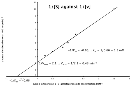
Hence, the final graph is:


If you didn’t understand that ‘mathematical move’ consider this:

The above is true. That is, 2 over 1 = 2, 4 over 1 = 4 and 2 times 4 is 8. If I simply invert (flip) all the parts:

It is also true.
Equation 3 is getting closer to what we want as we now have 1/v and this is our y in equation 1. All we need to do now is ‘extract’ x (which is our substrate concentration) from equation 3.
So, we have:

which is the same as:

If you consider the following it is true:
we can ‘separate terms’ on this and express it in several other ways:

That is, once we find a ‘common’ element (in the above example 1/2, and in equation 5 1 over [S]Vmax) we rearrange, so:

extracting 1 over [S]Vmax in equation 4 we get:

multiplying through with 1 over [S]Vmax gives:

As you can see in equation 6 we have two terms after the + that can cancel out, and our experimental variable (S) can be separated, so:
/div>

so we get:

If that bit of maths has lost you, consider this:
if you divide both sides by 2 it is still correct:

However, on the righthand side the two 2s can be cancelled to give:

which is still correct.
Finally, separating out 1/[S] from 7 gives:

Which when compare to equation 1:

It can be seen that:
- y = 1/v
- x = 1/[S]
- c, the y intercept = 1/Vmax
- m, the gradient = Km/Vmax
Hence, the final graph is:

If you would like to support my blogging efforts, then please feel free to buy me a coffee at https://www.buymeacoffee.com/drnickm
Additional Resources
- 📗 - Biochemistry (Stryer) (affiliate link to the book)
- 📗 - Principles of Biochemistry (Lehninger) (affiliate link to the book)
- 📗 - Maths and Chemistry Refresher for Life and Biomedical Scientists
- 📗 - Catchup Chemistry (affiliate link to the book)
- 📗 - Catchup Maths and Stats (affiliate link to the book)

No comments:
Post a Comment