Friday 11 December 2009

Why did I get my standard deviation calculation wrong?

A number of the class have asked why (or how) they got the standard deviation calculation wrong in the assessment.

Having looked at the class answers it would appear that the main reason students got it wrong is because they were calculating the standard deviation of a POPULATION and not of a SAMPLE.

The equation for the standard deviation of a population (remember a population is ALL possible examples of a measurement/object and is something that is normally difficult to measure - think of the apple example in the lecture - as all examples can't be collected) is:
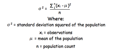
Standard deviation of a population

Equation for the standard deviation of a population

Whereas the standard deviation of a sample (which is what we had) is calculated by:

Standard deviation of a sample

Equation for the standard deviation of a sample

Note that the real differences between the two equation are that in the calculation of the standard deviation of a population we are using the true population mean (µ), whereas in the calculation of the standard deviation of a sample we are using an estimate of the mean (x bar), plus in the calculation of the standard deviation of a sample we are using n - 1 (also called degrees of freedom) as this gives better estimate of the true standard deviation of a population (and we are working with a sample).

Tuesday 1 December 2009

How many molecules of X are there in a band on a Western Blot?

One of the questions I have often enjoyed setting in western blotting assessments, and that always seems to give problems is....

"You have set up a western blot in which you wish to estimate the amount of GLUT4 per 3T3-L1 adipocyte (the cultured cell line used in the practical). You know that a 35 mm culture dish contains 2 million cells, and gives 1.5 mg total protein. You also have a recombinant stock of GLUT4 at 50 ng/ml. On your gel you load 15 µg of protein from the 3T3-L1 adipocytes and 1, 5, 10 and 20 µl of the GLUT4 stock. After probing with antibodies you have a 55 kDa band in the 3T3-L1 adipocyte lane, and in the GLUT4 stock lane. The band in the 3T3-L1 adipocyte sample has the same intensity of band as the 10 µl GLUT4 stock. How many molecules of GLUT4 are there per adipocyte?"

The chances are you are getting 'freaked out' by all the weird numbers flying around. The answer is to go back to basics.

For example:

If you had something with a molecular weight of 10, and you loaded 5 g on a lane, you would have 0.5 moles in that lane.

You know how many molecules there are in a mole (it is a constant that is the number of atoms in 12 g of carbon 12), so that constant multiplied by the number of moles, would be the number of molecules in the lane.

Let's say 1 mole of something contains 100 molecules (which it doesn't, the real number is much much bigger).

So, if you have 0.5 mole in the lane you would have 50 molecules in that lane.

If you have another lane with a known number of cells in, say 25, and that lane has the same intensity of staining as the lane containing 50 molecules you could say that lane also has 50 molecules.
These 50 molecules came from 25 cells, so each cell must have 2 molecules.....

Now you can work it through with 'simple' numbers all you need to do is to plug in the 'complicated' numbers in the question....

If you struggle with 'Science Maths' then you may like to look at: Maths4Biosciences

Monday 2 November 2009

Deriving Lineweaver-Burk Reciprocal Plot from Michaelis Menten Equation II

OK, well, here is another way Deriving Lineweaver-Burk Reciprocal Plot from Michaelis Menten Equation, this time starting from a different point (the other approach is here)...

Blog Post Bonus: Download a PDF of this blog post for your class notes.
The enzymatic reaction can be viewed as:


Enzymes equation


Where E = enzyme; S = substrate; ES = Enzyme substrate complex; and P = product

The Michaelis-Menton Equation given in your lectures describing the reaction is:


Eq2 2 1


Where v = rate (initial velocity); Vmax = maximum velocity (100% of enzyme catalytic sites occupied); Km = Michaelis constant (concentration of substrate to achieve half Vmax); S = substrate concentration

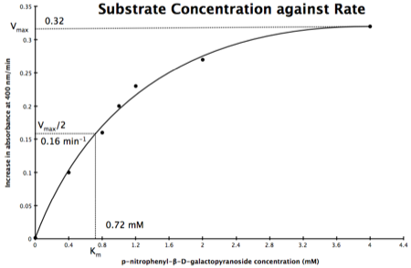
In the lab we can change the substrate concentration (S) in a reaction and measure the rate (v). As you know, a plot of substrate concentration (S) against rate (v; initial velocity) gives a curve, which plateaus at Vmax, with Km the concentration at half-Vmax:


Substrate concentration against rate


Plot of Substrate Concentration against Initial Velocity (rate)

The direct measurement for Vmax can never be achieved in the lab as the concentration of the substrate needed would never be reached. Also, in the lab we would use a computer to calculate the values, and determine Vmax, and Km. However, you should be able to calculate Vmax, and Km yourself, just so you know the computer is right, and it is possible calculate these values from experimental data by using a linear plot and an equation derived from the Michaelis-Menton Equation.

As you know, the equation for a straight line is:


Equation 1


Equation for a straight line, where m = the gradient and c = the intercept on the y-axis
So, the problem is, how do we get:


Eq2 1


to look like equation 1 so we can plot a straight line using the terms we can measure, i.e v and S? The answer is, we rearrange....

Blog Post Bonus: Download a PDF of this blog post for your class notes.
The first thing we need to do is invert equation 2 to get:


Eq2 3


If you didn’t understand that ‘mathematical move’ consider this:

Equation 4


The above is true. That is, 2 over 1 = 2, 4 over 1 = 4 and 2 times 4 is 8. If I simply invert (flip) all the parts:


Equation 5


It is also true.

Equation 3 is getting closer to what we want as we now have 1/v and this is our y in equation 1. All we need to do now is ‘extract’ x (which is our substrate concentration) from equation 3.

So, we have:


Eq2 4


which is the same as:


Eq2 5

If you consider the following it is true:


we can ‘separate terms’ on this and express it in several other ways:


Equation 12

That is, once we find a ‘common’ element (in the above example 1/2, and in equation 5 1 over [S]Vmax) we rearrange, so:


Eq2 5


extracting 1 over [S]Vmax in equation 4 we get:


Eq2 6


multiplying through with 1 over [S]Vmax gives:


Eq2 7


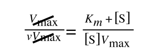
As you can see in equation 6 we have two terms after the + that can cancel out, and our experimental variable (S) can be separated, so:

/div>
Eq2 8


so we get:


Eq2 9


If that bit of maths has lost you, consider this:


Equation 9


if you divide both sides by 2 it is still correct:


Equation 10


However, on the righthand side the two 2s can be cancelled to give:


Equation 10a


which is still correct.

Finally, separating out 1/[S] from 7 gives:


Eq2 10


Which when compare to equation 1:


Equation 19


It can be seen that:
  • y = 1/v
  • x = 1/[S]
  • c, the y intercept = 1/Vmax
  • m, the gradient = Km/Vmax
And, the intercept for the x axis, (i.e. when rate (y) = 0) is 1/-Km.

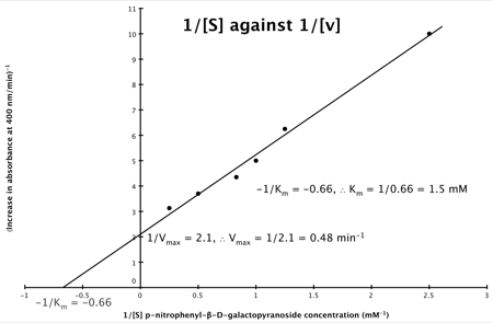
Hence, the final graph is:


Lbgraph


Blog Post Bonus: Download a PDF of this blog post for your class notes.
If you would like to test your skills at performing enzyme kinetics calculations then you might like to look at: Maths4Biosciences.com.

Sunday 1 November 2009

Deriving Lineweaver-Burk Reciprocal Plot from Michaelis Menten Equation I

After a recent seminar, a number of students have asked how to derive the Lineweaver-Burk Reciprocal Plot equation from the Michaelis Menten equation... so, here goes.

Blog Post Bonus: Download a PDF of this blog post for your class notes.
The enzymatic reaction can be viewed as:

Enzymes equation

Where E = enzyme; S = substrate; ES = Enzyme substrate complex; and P = product

The Michaelis-Menton Equation describing the reaction is:


Michaelis menton


Where v = rate (initial velocity); Vmax = maximum velocity (100% of enzyme catalytic sites occupied); Km = Michaelis constant (concentration of substrate to achieve half Vmax); S = substrate concentration

Now, if the equation you are starting with does not look like the one above then have a look at another post (apparently I do it the 'old fashioned way’!)

In the lab, we can change the substrate concentration (S) in a reaction and measure the rate (v). As you know, a plot of substrate concentration (S) against rate (v; initial velocity) gives a curve, which plateaus at Vmax, with Km the concentration at half-Vmax:


Substrate concentration against rate

Plot of Substrate Concentration against Initial Velocity (rate)

The direct measurement for Vmax can never be achieved in the lab as the concentration of the substrate needed would never be reached. Also, in the lab, we would use a computer to calculate the values and determine Vmax, and Km. However, you should be able to calculate Vmax, and Km yourself, just so you know the computer is right, and it is possible to calculate these values from experimental data by using a linear plot and an equation derived from the Michaelis-Menton Equation.

As you know, the equation for a straight line is:


Equation 1

Equation for a straight line, where m = the gradient and c = the intercept on the y-axis

So, the problem is, how do we get:

Equation 2

to look like equation 1? The answer is, we rearrange....

Rearranging

We need to 'extract' our substrate concentration S and our rate v so we can plot them on a straight-line graph. Basically, we need to get equation 2 to look like equation 1.

The equation for a straight line is:

Equation 1

And our Michaelis-Menton Equation:

Equation 2

So, the first thing we need to do is invert equation 2 to get:

Equation 3

If you didn’t understand that ‘mathematical move’ consider this:

Equation 4

The above is true. That is, 2 over 1 = 2, 4 over 1 = 4 and 2 times 4 is 8. If I simply invert (flip) all the parts:

Equation 5

It is also true.

Equation 3 is getting closer to what we want. However, the Vmax over v is a problem as we don’t know Vmax and can only measure v and S in the lab. Therefore, we need to separate out the terms we can measure so we can have x and y as in equation 1.

To ‘remove’ the Vmax from the lefthand side we need to divide both sides by Vmax:

Equation 6

Note the new Vmax term on both sides of the equation - compare to equation 3

Blog Post Bonus: Download a PDF of this blog post for your class notes.
As we now have Vmax over v multiplied by Vmax we can cancel out both Vmax:

Equation 7

to give:

Equation 8

If that bit of maths has lost you, consider this:

Equation 9

if you divide both sides by 2 it is still correct:

Equation 10

However, on the righthand side the two 2s can be cancelled to give:

Equation 10a

which is still correct.

In equation 5 we now have 1/v and this is our y in equation 1. All we need to do now is ‘extract’ x (which is our substrate concentration) from equation 5.

If you consider the following it is true:

Equation 11

we can ‘separate terms’ on this and express it in several other ways:

Equation 12

That is, once we find a ‘common’ element (in the above example 1/2, and in equation 5 1 over [S]Vmax) we rearrange, so:

Equation 13

extracting 1 over [S]Vmax we get:

Equation 14

multiplying through with 1 over [S]Vmax gives:

Equation 15

As you can see in equation 7 we have two terms after the + that can cancel out, and our experimental variable (S) can be separated, so:

Equation 16
Equation 17

Finally, separating out 1/[S] gives:

Equation 18

Which when compare to equation 1:

Equation 19

It can be seen that:
  • y = 1/v
  • x = 1/[S]
  • c, the y-intercept = 1/Vmax
  • m, the gradient = Km/Vmax
And, the intercept for the x axis, (i.e. when rate (y) = 0) is 1/-Km.

Hence, the final graph is:


Lbgraph

Blog Post Bonus: Download a PDF of this blog post for your class notes.
If you would like to test your skills at performing enzyme kinetics calculations then you might like to look at: Maths4Biosciences.com.